
Seagrass meadows are often described as simple habitats, composed of plants quietly photosynthesizing beneath the surface. Anyone who has worked in seagrass bed knows how misleading that image is. Seagrass ecosystems are shaped by constant light changes, moving water, mobile sediments, animals, and feedbacks that operate across minutes to decades. Understanding how these systems function requires more than knowing what to measure; it requires knowing how those measurements actually happen underwater, and what they really mean once you are back on land looking at the data.
This article is written from that perspective. It is informed by years of fieldwork in seagrass meadows, walking into intertidal beds at low tide, diving in subtidal meadows across the world with limited visibility, deploying and recovering instruments, losing sensors due to storms, cleaning fouled loggers, and adapting sampling designs to conditions that rarely match the plan. Many of the most important decisions in seagrass research are made in the field, yet they are often reduced to a single line in a methods section. This post exists to unpack what sits behind those lines.
Rather than presenting a catalogue of methods, this blog brings together the why, how, and what it tells us across key components of seagrass ecosystems: light, sediments, hydrodynamics, meadow structure, fauna, herbivory, and restoration. These elements are deeply interconnected. Light controls productivity, hydrodynamics shape sediments and canopy structure, sediments regulate nutrients and carbon storage, fauna mediate trophic and biogeochemical processes, and restoration and grazing alter feedback loops that can either stabilize or destabilize a meadow. Measuring any one component in isolation risks missing the system-level story.
This is not a review paper, and it is not meant to replace methods manuals or primary literature. Instead, it sits in the space between them. What you will find here are field-tested approaches, common analytical frameworks, key equations, and practical considerations that rarely make it into publications but strongly influence data quality and interpretation. The goal is to help readers connect measurements to processes, and tools to ecological meaning.
How to use this article: Each section can be read independently, depending on your interests or field needs. Basic equations are included as analytical reference points, and practical tips highlight common pitfalls and trade-offs encountered during underwater work. Whether you are a student planning your first field campaign, a researcher expanding into new measurements, or a coastal manager interpreting monitoring data, this post is intended as a practical, systems-based reference for working in seagrass meadows.
Underwater light: Quantifying irradiance
 Light availability is the primary factor controlling seagrass distribution, depth limits, productivity, and survival. Even modest reductions in underwater light can constrain photosynthesis, leading to reduced growth, increased mortality, and shallower depth limits, a relationship formalized by Dennison et al. (1993). Because underwater light is shaped by depth, turbidity, wave action, and canopy structure, quantifying the light environment is fundamental to understanding seagrass ecosystem functioning.
Light in coastal waters is highly dynamic. Daily and seasonal cycles, wave-driven sediment resuspension, currents, epiphyte growth, and changes in water clarity can cause strong variability over timescales ranging from minutes to months. Capturing this variability requires in situ measurements that reflect the conditions experienced directly by seagrass leaves and the sediment surface. Common research questions include:
- How much light reaches the canopy?
- How turbidity and epiphytes reduce irradiance?
- Which light thresholds define seagrass depth limits or restoration success?
In practice, we usually measure underwater Photosynthetically Active Radiation (PAR) at two depths above the canopy using submerged light loggers (e.g., HOBO, Apogee, LICOR, Oddysey). These are often paired with fluorometers (to estimate chlorophyll a) and/or turbidity or optical backscatter sensors (e.g., C3-Turner Designs) to help identify the main drivers of light attenuation, such as sediment resuspension or phytoplankton blooms. For instance, elevated turbidity with low chlorophyll a is consistent with resuspended sediments, whereas elevated chlorophyll a suggests turbidity driven by phytoplankton biomass. Simple tools such as Secchi disks remain useful for rapid assessments, but for long-term dataseries, deploying dataloggers are needed to resolve ecologically meaningful variability. Sensor placement relative to canopy height and the sediment surface is critical, as small vertical differences can lead to large changes in measured irradiance.
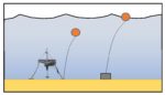
Practical considerations in the field include: deploying paired PAR sensors separated by a known vertical distance to resolve light gradients, see more details in the Blog post ‘Instrument deployment at sea’ ; regularly cleaning and calibrating sensors to minimize fouling effects; pairing irradiance measurements with turbidity and suspended sediment data to identify drivers of light limitation; using time-series data to calculate daily or seasonal light integrals for productivity estimates; and removing night-time measurements prior to analysis!!!
- Dennison WC, et al. (1993) Assessing water quality with submersed aquatic vegetation. BioScience, 43(2), 86-94
- Duarte CM (1991) Seagrass depth limits. Aquatic Botany, 40(4), 363-377
Measuring sediment properties: the story underneath
Sediments form the biogeochemical engine of seagrass meadows. Beneath the canopy, sediments regulate carbon sequestration, nutrient recycling, oxygen availability, and the chemical conditions experienced by roots and rhizomes. Grain size, porosity, and organic matter content influence how sediments store carbon and nutrients, while microbial processes control whether sediments act as sinks or sources of greenhouse gases and dissolved nutrients. Understanding sediment properties is therefore essential for interpreting seagrass productivity, hydrodynamic exposure, carbon sequestration, oxygen/sulphide conditions and habitat suitability for restoration.
Because these processes operate belowground and across multiple spatial and temporal scales, sediment research rarely relies on a single measurement. Instead, researchers combine physical characterization, porewater chemistry, and experimental approaches to capture the coupled physical, chemical, and biological dynamics that shape sediment functioning and its response to disturbance or restoration.
Sediment cores: Physical structure and carbon storage Sediment cores provide the primary window into the vertical structure of seagrass sediments. Extracting intact cores in dense meadows, where roots and rhizomes bind the sediment, requires careful technique and diver control, but yields critical information on how sediments are formed and maintained. Core analyses address questions such as:
- How much organic carbon and nitrogen are stored in seagrass sediments?
- How stable these stocks are over time?
- How sediment properties differ between natural and restored meadows or along hydrodynamic gradients?
From sectioned cores, researchers quantify grain size, bulk density, porosity, and organic matter content, often paired with elemental and stable isotope analyses (δ¹³C, δ¹⁵N) to trace carbon sources and diagenetic processes.
Porewater chemistry: Redox conditions and nutrient availability

Porewater measurements are used to quatify the chemical environment experienced by seagrass roots and sediment microbes. Dissolved nutrients, sulfide, oxygen, and redox potential reflect the balance between organic matter decomposition, microbial metabolism, and solute exchange with overlying water. Vertical porewater profiles help identify redox zonation, nutrient regeneration hotspots, and conditions that may limit plant performance or favor sulfide toxicity. Key questions include:
- What are the concentrations of dissolved nutrients, sulfides, and other redox-sensitive compounds in the sediment?
- How do porewater properties vary with depth, season, or meadow condition?
- How does microbial activity influence carbon decomposition and nutrient fluxes?
In practice, we sample porewater using long needles constructed from lab plastic pippetes. We drilled small holes into the pippetes and placed filter inside to avoid clogging with sediment. The pippetes were then connected with PVC tubing to syringes and inserted at defined sediment depths. Careful handling of porewater samples is essential to avoid oxygen contamination, pressure artifacts, or sediment disturbance that can alter measured concentrations. Another method to measure the presence of sulfide in the sediment is silver sticks, which provides rapid assessments.
Sediment incubations and benthic chambers: Process-based measurements
 While cores and porewater profiles describe sediment structure and chemical gradients, incubations and benthic chambers allow direct measurement of sediment processes. These approaches quantify rates of oxygen consumption, nutrient release or uptake, carbon mineralization, and gas exchange under controlled or semi-natural conditions. They are particularly valuable for testing how plants and sediments respond to changes in temperature, light, organic matter inputs, or restoration status. Common research questions include:
- How do oxygen consumption, CO₂ release, and nutrient fluxes affect seagrass productivity?
- How do changes in temperature, light, or organic matter addition affect carbon cycling?
- What is the effect of seagrass restoration on sediment biogeochemistry?
Practical considerations for sediment studies include: minimizing core compaction during extraction; aligning porewater sampling depths with root zones; pairing sediment measurements with hydrodynamic and light data to interpret drivers; accounting for spatial variability through replication; and recognizing that short-term process measurements reflect specific environmental conditions rather than long-term averages.
- Fourqurean, JW, et al. (2012) Seagrass ecosystems as a globally significant carbon stock. Nature Geoscience, 5, 505-509.
- Kennedy H, et al. (2010) Seagrass sediments as a global carbon sink: Isotopic constraints. Global Biogeochemical Cycles, 24, GB4026.
- Holmer M & Nielsen SL (1997) Sediment sulfur dynamics related to biomass-density patterns in Zostera marina. Marine Ecology Progress Series, 146, 163-171.
- Frederiksen MS & Glud RN (2006) Oxygen dynamics in the rhizosphere of Zostera marina. Limnology and Oceanography, 51(2), 1072-1082.
- Glud RN (2008) Oxygen dynamics of marine sediments. Marine Biology Research, 4(4), 243-289.
- Borum J, et al. (2005) The potential role of plant oxygen and sulphide dynamics in die-off events of seagrasses. Journal of Ecology, 93(1), 148-158.

Faunal communities: Epifauna, infauna, and fish
Seagrass meadows are structured not only by plants and sediments but also by the animals that inhabit them. Faunal communities integrate the effects of sediment, water movement, light, and canopy structure, serving as sensitive indicators of ecosystem health, habitat complexity, and restoration outcomes. Epifauna, infauna, and fish respond differently to environmental gradients, so sampling must be tailored to their ecology and behavior. Together, they provide information on trophic interactions, nutrient cycling, and ecosystem resilience.
Epifauna: Life on the seagrass leaves

Epifauna live on seagrass leaves and in the water column immediately above the canopy, and include small crustaceans, gastropods, and juvenile stages of many taxa. Their close association with canopy structure makes them highly responsive to changes in shoot density, leaf length, and epiphyte load. Common research questions include:
- How does canopy density and height influence epifaunal abundance and diversity?
- Do restored meadows support epifaunal communities comparable to natural systems?
- How does epifauna contribute to trophic transfer and nutrient cycling?
Epifauna are typically sampled using hand-held nets placed directly over the canopy, enclosure nets that isolate a known area, or tent-shaped passive traps that capture mobile organisms moving upwards within the meadow. Samples are usually rinsed through fine-mesh sieves (commonly 250-500 µm) to separate fauna from plant material and sediment. Subsequent taxonomic identification under a microscope is often the most time-consuming step, requiring expertise and substantial processing time, particularly for diverse crustacean assemblages.
Practical tips include standardizing sampled area or volume, and pairing epifaunal data with canopy structure measurements (e.g., number of shoots, leaf length, Surface area) to aid interpretation. If damage to the meadow is not allowed then enclosure nets work well, otherwise hand nets are more time efficient underwater.
Infauna: Organisms living within the sediment
 Infauna live within the sediment matrix and include polychaetes, bivalves, echinoderms, and other benthic organisms that strongly influence sediment mixing, oxygen penetration, and nutrient fluxes. Scientific questions typically include:
- How does infaunal community structure vary across sediment types and meadows, depth gradients or seasons?
- What role does infauna play in sediment biogeochemistry and carbon cycling?
- How do disturbance and restoration alter infaunal assemblages?
Infauna are collected using sediment corers of known diameter and depth, ensuring consistent sampling volume. Samples are washed through coarse to fine sieves (typically 500 µm or 1 mm), preserved, and later identified in the laboratory. As with epifauna, taxonomic identification is labor-intensive, often representing the largest investment of time in infaunal studies.
Data analysis commonly includes abundance, biomass, and functional traits, alongside diversity metrics. Infaunal studies increasingly rely on functional diversity indices, bioturbation potential indices, and multivariate community analyses, which better capture ecosystem functioning than species counts alone.
Fish: Mobile consumers and habitat users
 Fish are among the most visible components of seagrass ecosystems and are key indicators of habitat complexity, connectivity, and ecosystem services. Because fish are mobile and behaviorally responsive, sampling methods must carefully account for scale, visibility, and observer effects. Research questions commonly include:
- How does seagrass structure influence fish abundance, diversity, and size distribution?
- Do restored meadows provide habitat equivalent to natural systems?
- How do seagrass meadows function as nursery areas?
Fish are sampled using diver-based visual transects, underwater beach seines in shallow systems, or photogrammetry approaches such as stereo-video transects and static baited or unbaited cameras. Photogrammetry allows accurate length measurements while minimizing diver disturbance, but requires careful calibration and standardized protocols.
- Gagnon K, et al. (2021) Rapid faunal colonisation and recovery of biodiversity and functional diversity following eelgrass (Zostera marina) restoration. Restoration Ecology, 29(6):e13512.
- Orth RJ, et al. (1984) Faunal communities in seagrass beds: A review of the influence of plant structure. Estuaries, 7(4):339-350
- Heck KL, et al. (2003) Critical evaluation of the nursery role hypothesis for seagrass meadows. Marine Ecology Progress Series, 253:123-136

Measuring currents and waves
Water motion is a fundamental driver of seagrass ecosystem structure and function. Currents and waves regulate sediment transport, nutrient exchange, oxygen delivery, and the mechanical stress experienced by plants. By interacting with canopy structure, hydrodynamics create feedbacks that influence meadow stability, productivity, and resilience. Even subtle changes in flow regime can alter sediment deposition, resuspension, and biogeochemical fluxes, making hydrodynamic measurements essential for interpreting patterns observed in sediments, fauna, and plant performance.
Unlike light, hydrodynamics are often invisible and spatially heterogeneous, varying over seconds to seasons and across small spatial scales within a meadow. Measuring them underwater requires matching the instrument and deployment strategy to the research question, sampling resolution, replication, and risk. Key questions commonly addressed include:
- How does seagrass canopy height and density modify current velocity and turbulence?
- How do waves interact with flexible canopies to dissipate energy and stabilize sediments?
- What hydrodynamic thresholds lead to sediment erosion, plant uprooting, or meadow loss?
- How do hydrodynamic conditions differ between natural and restored meadows?
Measuring currents: Mean flow and turbulence

Currents transport dissolved nutrients, particles, and gases, and control exchange between the sediment, canopy, and overlying water column. Within seagrass meadows, flow is typically attenuated by plant stems and leaves, creating vertical gradients in velocity and turbulence (Nepf 2012). These gradients are central to understanding sediment trapping, oxygen fluxes, and nutrient delivery to leaves and roots.
In practice, Acoustic Doppler Velocimeters (ADV) are widely used to resolve three-dimensional flow and turbulence at fixed points within or above the canopy, while Acoustic Doppler Current Profilers (ADCP) provide vertical profiles of mean flow across the water column. In low-energy or shallow environments, electromagnetic current meters offer robust measurements close to the sediment surface. For comparative studies or broad spatial surveys, simple dissolution-based methods such as plaster balls (clod cards) provide relative estimates of flow exposure, trading precision for replication and safety. Field tips for current measurements:
- Position sensors above/below the canopy to capture flow attenuation by the meadow.
- Use sampling rates according to the flow scales (seconds for turbulence, minutes for mean flow, hours for waves).
- Consider high-resolution instruments at a few sites with simpler methods across many locations.
Measuring waves: Oscillatory motion and energy dissipation

In shallow and exposed seagrass meadows, waves often dominate hydrodynamic forcing. Oscillatory wave motion controls sediment resuspension, bed shear stress, and plant movement, particularly during storms. Seagrass canopies can attenuate wave energy, reducing orbital velocities and stabilizing sediments, but this capacity depends on canopy density, flexibility, and meadow extent.
Wave measurements typically rely on pressure sensors or wave loggers, which infer wave properties from pressure fluctuations. These instruments are relatively robust and affordable, allowing spatial replication, but do not resolve wave direction. ADCPs configured for wave analysis provide full directional wave spectra and detailed statistics, but are costly and logistically demanding. For relative assessments of wave-induced motion, accelerometers (e.g., HOBO loggers) can be deployed to compare exposure among sites, recognizing that these data are comparative rather than absolute. Field tips for wave measurements:
- Secure instruments carefully to prevent burial or loss during storms.
- Correct pressure-derived wave data for depth attenuation.
- Pair wave measurements with sediment and canopy data to interpret ecological effects.
- Use long-term deployments to capture episodic, high-energy events that drive change.
Analytical context and integration
Hydrodynamic data are often analyzed alongside sediment properties, light availability, and meadow structure to reveal coupled processes. While mean velocities and wave heights are informative, many studies increasingly use integrated metrics such as shear stress, energy dissipation rates, or attenuation coefficients to link physical forcing directly to ecological responses. Multivariate approaches and coupled physical–biological models are also commonly used to explore feedbacks between flow, canopy structure, and ecosystem function. By quantifying both currents and waves, researchers establish the physical template upon which seagrass ecosystems are built, allowing patterns in sediment dynamics, faunal communities, herbivory, and restoration success to be interpreted within a coherent, process-based framework.
- Fonseca MS & Fisher JS (1986) A comparison of canopy friction and sediment movement between seagrass species. Estuarine, Coastal and Shelf Science, 22(4):399-407
- Infantes E, et al. (2009) Wave energy and the upper depth limit distribution of Posidonia oceanica. Botanica marinae, 52:419-427
- Koch EW (2001) Beyond light: Physical, geological, and geochemical parameters as possible submersed aquatic vegetation habitat requirements. Estuaries, 24(1):1-17
- Nepf HM (2012) Flow and transport in regions with aquatic vegetation. Annual Review of Fluid Mechanics, 44:123-14
Quantifying meadow morphology and structure

Seagrass meadow morphology describes the physical structure of the plant canopy and is central to how meadows interact with light, water flow, sediments, and fauna. Most morphological metrics are intentionally simple: they are designed to be repeatable, scalable, and comparable across sites, species, and studies. These measurements form the backbone of condition assessments, restoration monitoring, and process-based studies. Practical tips for field application.
- Use quadrat sizes according to plant densities, for example too large quadrats at high densities will be very time consumming. Ensure enough replication.
- Measure morphology along transects to capture spatial variability by using measuring tapes.
- Pair structural metrics with light and hydrodynamic measurements to interpret functional effects.
- In restoration studies, track morphology over time (months, years), not just at a single snapshot.

Studying herbivory with cages: Protecting and exposing seagrass
 Herbivory is a key top-down process shaping seagrass structure, productivity, and recovery (Heck and Valentine 2006). Grazers such as fish, sea urchins, turtles, and waterfowl can rapidly remove aboveground biomass, altering canopy height, shoot density, and sediment stability. Quantifying grazing is therefore essential, particularly in disturbed or restored meadows where herbivory can determine success or failure.
Because direct observation of grazing underwater is difficult, herbivory is commonly assessed using cage experiments that selectively exclude grazers. Studies typically compare exclusion cages, partial cages, open cages (procedural controls), and open plots to isolate grazing effects while accounting for cage artifacts such as shading or reduced flow. Cages are deployed over small patches (≈0.25-1 m²) for weeks to months, with mesh size chosen to exclude target herbivores while maintaining water exchange. Non-destructive metrics such as canopy height reduction, leaf area loss, or shoot density change are often used when harvesting is limited.
Identifying the main grazers usually requires complementary observations, including visual surveys, underwater video, bite-mark analysis, or enclosure experiments with known grazer densities. Herbivory rarely acts in isolation: its ecological effects are best interpreted alongside measurements of meadow structure, light availability, hydrodynamics, and sediment conditions.
- Heck KL & Valentine JF (2006) Plant-herbivore interactions in seagrass meadows. Journal of Experimental Marine Biology and Ecology, 330(1):420-436
- Gera A, et al. (2013) Combined effects of fragmentation and herbivory on Posidonia oceanica seagrass ecosystems. Journal of Ecology, 101(4):1064-1075
- Moksnes, P‑O et al (2008) Trophic cascades in a temperate seagrass community. Oikos, 117(1):763-777
Seagrass restoration: From site selection to functional recovery
 Seagrass restoration is most successful when it is treated as a process-based experiment rather than a planting exercise. While initial survival is necessary, long-term success depends on whether restored sites meet the physical, chemical, and biological conditions required for meadow persistence and whether key ecosystem functions, such as habitat provision and carbon storage, begin to recover. Restoration monitoring therefore focuses on diagnosing why plants survive or fail, and how restored meadows transition toward natural systems. Key research and management questions include:
- Which light, sediment, and hydrodynamic conditions define suitable sites before planting?
- Which physical or chemical constraints (e.g. light limitation, sediment instability, sulfide accumulation) cause post-planting mortality?
- How quickly do restored meadows increase habitat complexity, faunal use, and biodiversity?
- When restored sediments begin to accumulate blue carbon and at what rate?
In practice, restoration studies integrate a small set of highly diagnostic measurements. Structural metrics such as shoot density, canopy height, patch size, and percent cover are tracked alongside underwater light, temperature, salinity and hydrodynamic exposure. Together, these measurements identify whether failure is driven by physical stress (e.g. erosion, burial), chemical stress (e.g. sulfide toxicity), or biological interactions (e.g. herbivory). Effective restoration monitoring therefore emphasizes diagnostic simplicity, which are repeated measurements of a few key parameters (eg. shoot density), interpreted within the physical and biogeochemical context of the site. When combined with faunal surveys and sediment analyses, restoration becomes a powerful tool for understanding not only how to rebuild seagrass meadows, but which processes ultimately sustain them.
- Orth RJ, et al. (2006) A global crisis for seagrass ecosystems. BioScience, 56(12), 987-996
- van Katwijk MM, et al. (2016) Global analysis of seagrass restoration: The importance of large-scale planting. Biological Conservation, 186:92101
- Moksnes, et al. (2016) Handbook for restoration of eelgrass (Zostera marina) in Sweden, National guideline. Swedish Agency for Marine and Water Management, Report 2016:9
Read about other research topics


Further reading on seagrass ecology


Related research articles


62. Successive stressors alter microbiome composition and reduce resilience in the eelgrass Zostera marina


Leave a Reply